Navigation

Previous
Next
Homepage
FAQ
What's new
Sitemap

Topics

Excel
Office button
Home
Insert
Page Layout
Formulas
Data
Review
View
Developer

Excercises
Autosum
Chart - Insert a second axis
Create a half-moon chart
Create a demographics chart
Conditional formatting
Data table
Goal Seek
Pivot table
Scenario Manager
Solver

Tutorials

Word
Excel 2003
Excel
PowerPoint
Access

Others

Demonstration files
Texte en français

Contact

By e-mail
Join our Newsletter

Share this page

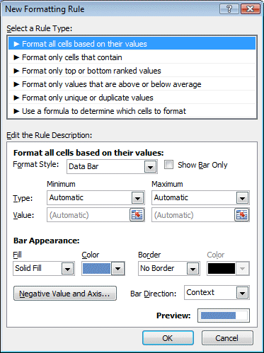
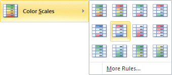
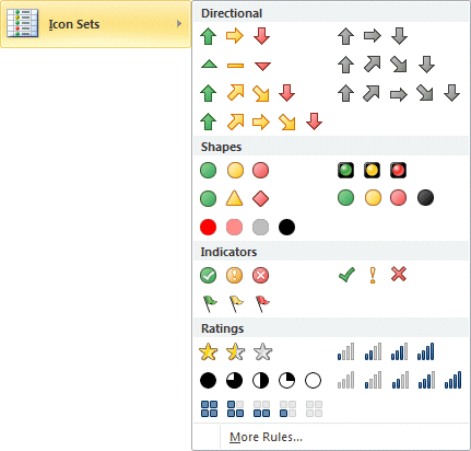
Excel/2010 - Exercises on Conditional formatting

Introduction
Before we start
Conditional formatting
Copy a conditionnal formatting
Data bars
Color scales
Icon sets

Introduction

Excel can change a cell's presentation according to the rules that you determine. You can change a cell's color, border color or style and a text's font size, type and color. The modification can be viewed immediately a good thing since a change in a value can have a serious impact on your results.

Microsoft greatly improved this option with Excel and made a few "tweeks" with Excel 2010. Not only can you change a cell's presentation, you can also represent values with horizontal bars (data bars), place a color scale (or heat map) or with sets of icons. These options were only found in specialized software before Excel.

This page contains many exercises to show you how to apply all the options under the conditional formatting button.

Before we start

To follow this exercise, you can use the file excel2007-2010-exercises.xlsx on the demonstrations files web page.

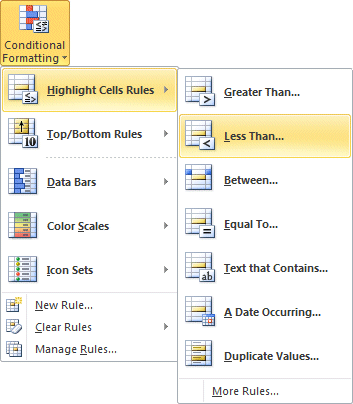
Select the Conditional formatting worksheet.

Conditional formatting

The first exercise will show you how to use the conditional formatting as it was available in the earlier versions of Excel. The newest options will come after.

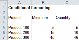
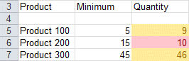
For this example, we will manage a small inventory. The text in the first column (A) contains the names of the products. The values in column B are the minimal values that must be in stock. The values in column C are the current quantities in inventory. You must reorder new items every time the current inventory falls below the minimal value for that item.

You can look at the two sets of values, analyze it and determine what product must be reordered. But it would be easier if something would "pop" on the screen when it's time to reorder. It's possible, if you apply for conditional formatting rules.

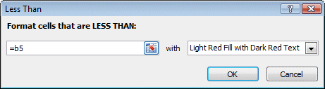
The first rule that will be applied is to turn the cell with the quantities in inventory to red when its value is less than the minimal quantity allowed.

Place the cursor in the C5 cell.
From the Home tab, press the Conditional formatting button.
Select the options Highlight Cells rules and Less Than …

In the LESS THAN box, write =B5 (and not =$B$5. The absolute reference would block the advantage of copying this rule later).
For this example, select the Light Red Fill with Dark Red Text style..
Press the OK button.
Change the value of the C5 cell to 3.

The rule will be activated since the value is lower than the content of the B5 cell. You can apply many rules to the same cell. The next example will change the cell's color to yellow when the value is close the minimal value. In this case, if the value is close to 5 (minimal value), it will turn to yellow to warn you that this item will need reordering soon.

Place the cursor in the C5 cell.
Select the options Highlight Cells Rules and Between …

In the first box, enter =B5.
In the second box, enter =B5+4.
From the list of styles, select Yellow Fill with Dark Yellow text.
Press the OK button.
Change the value of the C5 cell to 9.

Enter other values in the C5 cell to view the result.

Copy a conditionnal formatting

One of the conditional fromatting's strong point is that you can copy the rules and apply them to other cells. This is much easier than to redo them everytime. And it's also very easy to do.

Place the cursor in the C5 cell.
Under the Home tab, in the Clipboard group, select the Format Painter button.
Copy the format to the C6 and C7 cells.

The conditional formatting rules that you copied will only work if you removed the " $ " from the cell's references. If you do not remove it, the rules will always be compared to the content in the $B$5 cell (B5) instead of the cell to the left of the cell with the conditional formatting. Like the formulas, the conditional formatting rules also take into consideration the relative and absolute references rules ($).

Data bars

A new option that was added in Excel is the data bars. They represent a data from range of cells with a horizontal bar. It enables you to easily compare the values in the range. Excel 2010 offers more presentation styles for this option. The next example will use the grade average from five students to help you compare one grade from the others.

Select the range of cells G12 to G16.
From the Ribbons' Home tab, select the command Conditional formatting and Data bars options.

Select one of the color styles of your choice.

This option draws a horizontal bar to represent each value and help you compare the results. You don't even need to create a chart to know who has the best and the worst results. The Data Bars helps you to see the results before you can read the values. Enlarge the G column and view the result.

From the Ribbons' Home tab, select the command Conditional formatting and Data bars and the More Rules options.

you're not limited to one style in the Conditional formatting menu. From this window, you can change the format style, minimum and maximum values to represent, the styles (3 or 3 color scale, data bars, or icon sets. You can apply many formatting rules at the same time. The Data Bars adjust themselves to the new column's length. For the moment, press the Cancel button.

Color scales

Another option that was added with Excel is the capability to represent values with a color scale. Others have used the term "heat map" to explain this option. The next example consists of placing a color scale on all the student's grades.

Select the range of cells from B12 to F16.
From the Ribbons Home tab, select Conditional formatting  and the Color scales options.

	Select the color scale of your choice.
	You can see the values and compare them to each other just by looking at the colors in each cell.

Icon sets

Another way to represent the values is by using icon sets. Excel 2010 offers many sets to choose from. The next exercise consists of placing an icon set on a series of values.