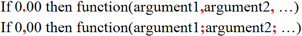
IntroductionThe biggest advantage of functions is that they are ready to be used. You don't have to recreate them or to look for them in books to find the one that you need. Excel's help file can help you find what you need. You just need to press the F1 key to have access to it. Be careful! This applies to all functions. The argument separatorAs much as I love Excel, there is one very nagging thing I just can't bear. It's the different argument separators. Most Excel functions need one or more parameters to work properly. Excel calls these parameters an argument. An argument separator is needed to separate the information required by the function. But Excel designers dropped the ball on this one. The argument separator is different depending on where you're located in the world. For example, if the decimal point is a period (.), then your argument separator will be a comma (,). That's what you'll see in most training videos. But, for most of the world, the decimal point is a comma. Therefore, the argument separator had to be changed. The semicolon (;) was used to replace the comma. That's what you will find in the instructions on this page and on the other pages on this website. Another way to look at it's ...
Just make sure that you're using the correct argument separator whether you're looking at this website or any other. Be careful! Exercices on simple functionsTo complete the next functions, fill in the cells with numbers and text in the appropriate cells.
The Sum function and the AutoSum button The =sum function is very probably the one most often used function
The result should be 600.
The new sum will be displayed in B5 cell. There are several ways of writing a formula. You can write a formula by writing it manually or by using the cursors or the mouse to select the proper cell that you will need in the formula. The next three exercises will demonstrate how to use these three techniques to find the sum between the B1 to B3 cells. Once you've have mastered these techniques, you can use them for any functions and formulas.
You can always start a formula with the +, - or = mathematical operators.
Please notice that there is a box around the cell that flashes. It's to reassure you that you selected the right cell. You can't confuse it with the other cell on your worksheet.
Noice that the cursor returned to the B5 cell, where it will continue to write the formula. As soon as you press one of the mathematical operator keys (+,-, *,/, ^) or a bracket, the cursor always returns to the cell where it's writing the formula.
The formula is finished. The B5 cell will show the result of the formula. That's one way to write the formula. It's an easy way to write a formula if you don't have many cells to add up. But it may be the only way if you're using many different mathematical operators. For example, the sum() function won't be of any use to write this formula: =b1*(1+b2)/b3. The next exercise consists adding the same cell using the sum() function and by selecting an area of cells using the cursors.
The block is selected. The Shift key allows you to select a range of cells on witch you can do some operations. That can be from using them in a formula, changing their presentation or even deleting their content. You can do an operation on many cells instead of just one.
As just demonstrated it's also possible to select an area of cells by using cursors and the Shift key. You can have the same result by using the mouse. That's the next exercise.
This last exercise demonstrates that you may select an area of cells as much with the mouse as with the cursor keys. The AutoSum button is much simpler. But, it has its limitations you should be aware of.
Excel will offer you the formula: the sum of the B1 to B4 cells or =sum(B1:b4).
But how did the function determined the right area? The AutoSum function first looks upward to determine if there are any numbers to add up. If there are no numbers in the two cells directly above the active cell, the AutoSum will try to find numbers to the left of the cell. In the example above, it does not find numbers in the B4 cell just above. But it does find a number in the B3 cell. The function moves up the column until it finds an empty cell. At that moment, it stops and suggests you an area (=sum(B1:B4)). This option is very practical. The problem is that it can stop at the wrong place. If you have a cell that's empty from the block, the function will stop there, even if you wanted to have the other numbers above that empty cell. Be sure that the function selects the right area of cells before confirming by pressing on the Enter key. =Average(range of cells ex.: A1:D5)Finds the average for an area or range of cells.
VIDEO on Min(), Max(), Small(), Large(), Rank.eq() and Rank.avg()=Min(range of cells)Finds the smallest value among an area of cells.
=Max(range of cells)Finds the highest value among an area cells.
=Small(range of cells;N value)From a range of cells, you can fid the N smallest value. For example, you could enter 1 to find the smallest value. But you could also enter 2 to find the second smallest and so on.
That will find you the second smallest value from the range of cells selected. The Min function could not find that. =Large(range of cells; N value)From a range of cells, you can fid the N highest value. For example, you could enter 1 to find the highest value. But you could also enter 2 to find the second highest and so on.
That will find you the second highest value from the range of cells selected. The Max function could not find that. =Rand()This function generates a random number between 0 and 1. It's often used during simulations. You can change te random number by pressing the F9 key. You can also combine this function with other to make it more useful. The next example generates a number between 700 and 1000. The lowest possible value is 700 and the maximum is 1000. The difference between them is 300. You can use one of these formulas to generate a number between 700 and 1000: =ROUND((RAND()*300)+700,0) or =INT(RAND()*300)+700 . The function used in combinason with =rand() will be explained later on this page. =Abs(cell or value)Shows the absolute value, or positive value, of any number.
=Round(cell,number of decimals)Allows to round a number to the decimal place of your choice. You must enter the number, or the cell address where the number is located, and the number of decimals you need.
You can also round to the unit, to tens or the hundreds and so onby putting a negative value on the number of decimals. Ex.: =round(45,-1) = 50 These options also applies to the next two functions. =Roundup(cell,number of decimals)This function rounds up a number at the decimal place of your choice. A value will be rounded up even if there is just a faction after the decimal of your choice.
=Rounddown(cell,number of decimals)This function function "removes" any fraction after the decimal place of your choice.
=Int(cell)Shows the Integer of a value. It removes all the fractions after the decimal point.
=fact(number)Shows the factorial of a number. It's very useful calculating propabilities. Ex.: =fact(3) = 6 (1 * 2 * 3) =mod(number,divider)Shows what remains of a division. Ex.: =mod(13.4) = 1 .Thirdteen (13) divided by 4 is equal to 3. It remains 1. =count(range of cells)Counts the number of cells with a number, not text or empty, within a selected range of cells. =counta(range of cells)Counts the number of cells that have some content, that are not empty. The can either have numbers, text or formulas. =countif(range of cells,criteria)Counts the number of cells that have the same content as the criteria. The next exercise shows the number of cells that contain the number 100. The formula entered in the B1 cell is =countif(A1:A3,100) .
The result of the =countif() now shows that two cells contain the number 100. It's also possible to use this function to find if there are any other cells within a range that have the same value. You mus t combine the =countif() with the =if() function. The formula is =if(countif(range of cells,criteria)>1,"Double","Unique") .
For this example, the formula checks if the number that's in the A1 cell appears more than once within the range of A1 to A3. If that's the box, the result will show "Double". =sumif(range of cells,criteria)This function adds numbers that have the same value.
With this example, the function will add all the cells in the range that have the number100. Since there are two cells with that number, the result will be 200. =countblank(range of cells)Counts the number of empty cells in the selected range of cells. =even(number)Shows the next even number if the number isn't already even.
=odd(number)Shows the next odd number if the number isn't already odd.
=sqrt(number)Shows the square root of a number or from the content of a cell. Ex.: =sqrt(9) = 3 =sign(number)At times, it's useful to know not the value of a cell but it's sign. This function shows 1 if the number is positive, 0 for 0 and -1 for a negative value. The equivalent could be done with this formula =if(number>0,1,if(number=0,0,-1)) .
=trunc(number,number of decimals)Shows the number with the number of decimals desired. It's the equivalent of the =rounddown() function. Functions that applies to textExcel also has some functions that can help you get more out of the content of text cells. Here are some examples. =right(text,number of caracters)Shows the n caracter from the right of a cell with text. ex.: =right("This is an example",2) = le =left(text,number of caracters)Shows the number of caracters from the left of a cell with text. Ex.: =left("This is an example",2) = Th =concatenate(first cell,second cell)This function allows you to group the content of many cells together even if it's as different as text numbers dates or the result of a formula. Ex.: =concatenate("The",45) = Ce45 =len(cell or text)Shows the number of characters in a cell. Ex: =len("abcde") = 5 =roman(number)Converts a number to its roman equivalent. Ex.: =roman(45) = XLV =text(number,text format)Converts a number into text format. It will take the formatting as any other cell containing text. It's still possible to use the content for mathematical operations or in formulas. Ex.: =text(45,0) = 45 but the text is placed on the left border of the cell. Insert a function that applies to dates or timeExcel also offers functions that allows to get information on cells containing dates and time. These cells contain a lot of information. Here is a list of the functions of this category that most often used. =now()Shows the exact time at the moment you confirmed the content of the cell. It will also update itself every time you enter or change a value in a cell. =today()Shows the computer's date, whether is right or not. =year(cell with a date)Shows only the number for the year that's inside a date. =month(cell with a date)Shows the month that's inside a date. The result will always be between 1 and 12. =day(cell with a date)Shows the number of a day that's inside a date. The result will always be between 1 and 31. =workweek(cell with a date)Shows a number that represents a number for the day of the week: 1 = sunday, 2 = monday ... 7 = saturday. You can combine this function with =if() or vlookup() to show the day of the week instead of just a number. =hour(cell with time)Shows the hour that's inside a date or a time. The result will always be between 0 and 23. =minute(cell with time)Shows the minutes that's inside a date or a time. The result will always be between 0 and 59. =second(cell with time)Shows the seconds that's inside a date or a time. The result will always be between 0 and 59. Insert a functionLet's take the following example. You want to know how much will be your monthly payments if you take a 25 years mortgage at an annual rate of 6,5 %. There is already a function in Excel to help you to find the .
These formulas deserve a few explanations. The rate should be that for each payment periods and not the annual rate. To find the number of payments, you must multiply the number of years with the number of payments made during a year.
The PMT function window of the will appear. It shows the boxes that need information for the formula to work. The titles that are in bold (rate, number of periods and present value) are required. The titles that are of standard size (Fv and Type) are compulsory. You must enter the s in the boxes or to indicate the function in the cell that will find wanted s. For the exercise, it will be boxes B2, B3 and B1 respectively. The function window disappears. A smaller window with only the information on rate is shown. You must now choose the cell where the rate for the loan is contained.
The result of the function should be -337.60 $. To avoid the negative , you can put the - (minus) sign in front of the function (-PMT (...)) or in front of the of the mortgage (B1). You can now change the s and the rate to better suit your needs. You'll be able to better plan the you need to buy your first house. Don't forget to add to that, as a home owner, you'll have property and school taxes to pay, maybe a water tax and home maintenance cost that you didn't have before. Excel offers you several other functions in different categories. Experiment with these before needing them in your work. These functions help you to create models that are closer to reality. The IF function allows you to adapt the model according to different situations. For example, is there a premium to be paid? Are there overtime hours to be paid? =IfThe =If function is very practical in a model because it gives you can adapt your model to different situations. For example:
The number of possibilities is infinite! The other functions, with the exception of =Vlookup and =Hlookup, don't offer what this function can offer: a choice, some flexibility for your model. It will give a certain result if the condition is realized. Otherwise, another result will appear. The =If function requires three parameters to work. The first is the condition: what does it have to compare? The second part is what the function should show when the condition is true. The third part is what the function should show when the condition is false. You can summarize this: =If(condition, if true, if false). The semicolon (,) is used to separate the various parameters of the function. That's also true for every other function in Excel. Ex: =If(B1>=10,b3*0,1,0) If the contents of the B1 cell is superior or equal to 10, show B3's result multiplied by 0,1. Otherwise show zero. To help you understand how the =If function works, and its potential, the next part will have some exercises for it. This is the box of a businessman who wants to offer a discount to its customers if they buy a certain quantity.
For the first example, the businessman wants to offer a still undetermined discount if the customer buys 10 identical items or more. This exercise is just to show whether or not the customer has a right to a discount or not. The result of this =If function will only be text, not a number or a formula. Those will come later.
According to the quantity that's entered in the B1 cell, the B6 cell will show either "Discount" or "Sorry, no discount " (without quotation marks). As mentioned before, this function has the three parts. In the first part, B1>=10 is the condition. It verifies that the contents of the B1 cell is superior or equal to 10. If true, the function shows the second part of the function (Discount). Otherwise, it shows the third part (Sorry, no discount). The result of this function is posted as text. The next function will have for result a formula or a number.
The businessman has decided to offer a 10 % discount to those who buy 10 identical items or more. The next formula will calculate this discount.
For this formula, the condition is the same that the previous formula. Nevertheless, the result is different. The discount will change according to the quantity in the B1 cell. If the quantity equals or higher than 10, there will be a 10 % discount on the total in the B3 cell. Otherwise, there is no discount. So, the number will be zero ( 0 ).
The third exercise consists of seeing the =If functions been linked. It's possible to have if() functions inside a =If () function. In fact, you may have functions in functions. For example, =abs(sum(B1:B200)) gives you the absolute number of the sum of B1 to B200 cells. It's possible to imbricate up to six if() inside each other. The next exercise gives you the example of this. The businessman notices that his discount does not make any sense to most clients. They don't buy that many. He then offers a 5 % discount to those who buy 5 identical items or more. He also wants to give a 10 % discount if a customer buys 10 identical items or more.
The function verifies first if the quantity registered in the cell is superior or equal to 10. If true, the function will show a 10 % discount on the number in the B3 cell. Otherwise, there is the second if() that verifies if the quantity is superior or equal to 5. If true, it will show a 5 % discount on the number of the B3 cell. Otherwise, there is no discount. So, the shown number will be of zero ( 0 ). There is another possible formulation that would have given the same result. =If (B1>=5,if(B1>=10, b3*0,1,b3*0,05),0). Instead of beginning with the biggest possibility (>=10) and decent from there, this formula begins with the smallest possibility (>=5) and rises! There are certainly one or two other formulations that are possible. It's possible to " imbricate" up to 6 levels of Ifs. But at that level, it becomes very difficult to manage. The =Vlookup and =Hlookup functions will be easier to use when you have several possibilities. The function =If () can be improved when it's used with other functions such as =And() and =Or() . The next part demonstrates the functioning of these two functions followed of how they can be used with =If().
It's time see them in practice.
With these numbers, you should see the "FALSE" in cells B1 and B2. The numbers don't answer the conditions in either formula. For the = And() function to work, the cells A1 and A2 must be equal to 1, the necessary conditions for that function to be true are not yet met. It's the same situation for the =Or() function.
This should bring a change to the =Or() function because one of both conditions is realized. The B1 cell still shows false because all of the conditions are not yet met.
Because both conditions are now true, the =And() function will now show TRUE.
The result was predictable. The B1 cell shows false whereas the B2 cell will still shows true. If you want, you can add other conditions to these functions. Here is a small example: =Or(A1=1, A2=1, A3=1). This can go far, very far. It's possible to add these functions, and many others, in the =If() function. For these last two functions, it's better place them in the part of the conditions. =If(and(a1=1,a2=1),1000, 0) Video on the If() function and cell referencing=Vlookup, =HlookupThe =Vlookup and =Hlookup functions are forms of the =If function that are a little more developed. It's possible " to imbricate " up to 6 if functions to answer several possibilities. But what can you do if you want to answer a question that needs more than 6 levels? At that level, it becomes difficult to manage every imbricated =Ifs. It's easier at that point to use a Vlookup or Hlookup function especially when you have a grid or a comparison table ready to use. For example, using a grid to determine a student's grade or the grid to determine the tax rate of the employees. The Vlookup function uses a vertical comparison table were a Hlookup function uses a horizontal grid. Let's resume the last exercise of the =If function. A businessman gives a 5 % discount to customers who buy 5 of the same item or more. The discount is raised to 10 % if the customer buys 10 or more. Using the =If function, the formula may look like this: =If(B1>=10, b3*0.1, if (B1>=5, b3*0.05, 0)). This formula is simple because it has only three possibilities (10 and above, between 5 and 10 and between 0 and 5). The formula becomes more difficult to create when you add more and more possibilities. The function =Vlookup or =Hlookup can help in this situation. These functions need three parameters to work. The first one is the cell address that will be compared to a grid or a comparison table. It will be compared with the contents of the second argument that will contain the address of the range of cells of a comparison table. The third argument is to indicate the column (for =Vlookup) or the row (for =Hlookup) that will be shown from the comparison table. =Vlookup(cell to compare, comparison table, index of the column) Before using the function, you must prepare a comparison table.
The first column of the comparison table is used to compare with a cell that contains a number. The numbers of that first column must always be in ascending order. You always put in the lowest possible number, or the floor, to reach this level. The "ceiling" is the "floor" of the next row of the comparison table. So, for the first row of the table, the minimal number is zero whereas the maximum is 5 exclusive or [0 , 5[ for those that remember their mathematical operations. It's as for that reason that the numbers should always be in increasing order. So, for the table in the A11 to B13 cells, the number 0 of the A13 cell is the floor. The ceiling is the contents of the A12 cell, or 5. So for all numbers between 0 and up but not including 5 ([0 , 5[) will be on the first row of the table. It's infinitely close to 5 but it's not 5. All that's between 5 and infinitely close to 10 ([5 , 10[) will be on the second row. For the numbers equal or superior to 10, it will be the third row of the table. Because there are no other rows over the 10 of the A13 cell, the "ceiling" is infinite. The second, the third and the other columns usually contain the results that you want to show. For this table, the second column contains the discount rates according to the quantity that was bought.
According to the quantity that entered the B1 cell, the =Vlookup function will compare this to its comparison table. When it will know the row to stop, it can then show the appropriate content from the chosen column. For example, if the number is 6,5, the =Vlookup function will stop at the second row of the table (between 5 and 10). It will then show the contents of the second column of this row witch is 5 %. To help you to understand, here is another exercise with a grid for school grades. This exercise consists at showing the appropriate letter for a given note in the B2 cell according to the grade located in the B1 cell.
The B1 cell will contain the number of the grade. The B2 cell will contain the =Vlookup function that will compare the number in the B1 cell and will show a letter that's the equivalent to the grade. The B3 cell will contain a =Vlookup function that will compare the grade with the comparison table and show the appropriate comment. The A5 to B9 cells contain the comparison table. The table indicates that the letter will be an " e " if you have a grade below 50. Between 50 and 60, the grade will be a " d ". Between 60 and 75, the grade will be a" c ". Between 75 and 85, the grade will be a" b ". And, for a grade of 85 or more, the grade will an " a ". For the =Vlookup function to work correctly, it needs three parameters: the cell address to compare (B1), the place of the comparison table ( A4:B8) and the column to be shown with the result (the second column or 2)
You can also copy the formula into the G3 to G6 cells to find the grades noted in the F3 to F6 cells. Don't forget to "fix" the position of the comparison table by placing a "$" in front of the rows in the formula. Or else the formula will not work. You'll learn more about copying formulas and relative and absolute reference on the next Web page. We will continue with something more difficult for the =Vlookup function. It consists in using the =Vlookup function with two variables. The first variable is identical to what you saw before. The second variable consists of changing the comparison table column that in witch the function fetches the information to be shown.
Can you write the appropriate formula for the H2 cell? Write the formula that will show the comment in the H2 cell. Up until now, you always wrote the number 2 for the third argument of the =Vlookup function. The function always fetched the information to be shown in the second column of the comparison table. The next exercise consists in changing in the number in that column so that the =Vlookup function fetches the information to be shown according to the type of customer. That will be the second variable for this function. For this exercise, there are three categories of customers: type 1 , 2 and 3. The function should look for the information to be shown in the second, third or fourth column of the table, depending on the type of customer + 1 because the first column of the table is used to compare the quantities bought in the comparison table to determine the quantity of the discount.
You now have a new comparison table that takes into consideration the quantities bought and the type of client. The percentage of the discount will vary depending on the quantity and the type of client. The D1 cell is also important because it now defines the type of client being served.
Try the following combinations of numbers in B1 and D1 cells.
All the numbers work except for the last two boxes. In the first box, the bought is a negative quantity, this is smaller than the minimal threshold of the first row of the comparison table ( 0 ). So, this number does not apply to the comparison table. For the last box, the function tries to look for information that's outside of the comparison table. The table consists of four columns. But, the =Vlookup function looks for information in the Fifth Column, there is no data there. Video: Vlookup function and cell referencingTo make the =Vlookup or =Hlookup function even more powerful, it's also possible to use it to compare text. The first column of the comparison table can contain words instead of numbers. As for numbers, the list must be in ascending order. Contrary to numbers, the text should be exact. For example, the text can not be between Anjou and Avignon. Otherwise, you should expect the bizarre results as you'll see below.
The result will be 83 % in the B2 cell. You should expect in bizarre results when you use text. Let's look at other possibilities.
The result will be 99 %! Why? That's because it's listd after Paris. So, the function goes to the last row of the comparison table.
The result of the B2 cell will be 74 % because it's between Bern and Brussels. So, although the function is very practical to compare numbers, it may not be as appropriate for text unless you use the fourth pamateter. The fourth argument of this function is used to determine if the function sould look for an exact value to compare or be between two values. By default or when the fourth paramater equals 1, the function is comparing between numbers. When its value is 0, the function will look for an exact match.
The function will give you a "Not applicable" (#N/A) result because it's now looking for an exact value and not finding it. Boston is not in the comparason table. |

 button.
 And
And