Navigation Topics Tutorials Others Contact |
Excel - QuizIntroduction IntroductionThis page contains a little quiz to see what you learned from this site. They are all multiple choice questions. Only one answer is correct. The answers come after all the questions. Good luck! The quizQ1: What does this button mean?
|
|
Q2: What type of chart is this?
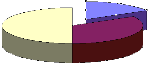
A: Doughnut
B: Radar
C: Bar
D: Pie
Q3: If you copy the formula =$B38 into another cell, the result will be:
A: The column part will remain the same
B: The row part will remain the same
C: Both the column and row will remain the same
D: Both will change
Q4: What will be the formula in the C5 cell if you want to copy it the the cells just below?
A: =$C3/B6
B: =C$3/B6
C: =C3/$B6
D: =C3/B$6
Q5: What tool is used to split the window into different parts of the same worksheet?
A: The title bar
B: The scroll bar
C: The toolbar
D: The split box
Q6: What is the combination of keys required to come back to the top of the worksheet?
A: PageUp (PgUp)
B: Alt and PageUp
C:CTRL and Home
D:CTRL and left arrow
Q7: What key is used to select multiple ranges of cells?
A: Shift
B:CTRL
C: Alt
D: AltCar or AltGr
Q8: What key should be used to change the content of a cell?
A: F1
B: F2
C: F3
D: F4
Q9: This button  represents:
A: The AutoCorrect button
B: The AutoFormat button
C: The AutoSum button
D: The conditional format button
Q10: What is the most appropriate formula you can put in the C2 cell to calculate a 7% tax?
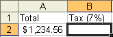
A: =A2*0.07
B: =A2*7%
C: =A2*1.07
D: =A2+(A2*0.07)
Q11: What function offers you the possibility to view different results depending on the entered condition?
A: =If()
B: =Sum()
C: =SumIf()
D: =TrueFalse()
Q12: What function is used to make sure that all conditions are true before showing a TRUE answer?
A: =AND()
B: =OR()
C: =Vlookup()
D: =If()
Q13: Which of these three functions will give you TRUE as an answer?
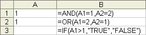
A: =AND(A1=1;A2=2)
B: =OR(A1=2;A2=1)
C: =IF(A1>1);"TRUE";"FALSE")
D: None of the above
Q14: Which of these statements on Vlookup() is false?
A: The Vlookup function can be used to compare a value that's between two values or for an exact value.
B: When this function is used to find a value between , you must always place the smallest possible value first in the first column.
C: The values of the first column must be in descending order.
D: With this function, the comparison table is always read vertically.
Q15: What will be the result according to this formula: =vlookup(B1;A4:B8;2) ?
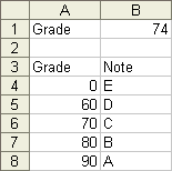
A: A
B: B
C: C
D: D
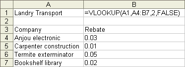
Q16: What will be the result from this vlookup() function?
A: 1%
B: 2%
C: 3%
D: 5%
E: None of the above
Q17: What tool helps you to optimize the results of a model?
A: Scenario manager
B: Solver
C: Target value
D: None of the above
Q18: True or false: The values that I enter in the scenario manager have an impact on my model.
A: True
B: False
Q19: Which button or command doesn't copy the content of a cell or a range of cells?
A: The button ![]() or
or ![]()
B: The Copy option from the context menu
C: TheCTRL and C keys.
D: None of the above
The answers
You answered all of the questions above. Let's see how well you've done. Most answers will also have a how about the option that was covered.
A1: C: Fuse the selected cells into one.
Excel allows you to fuse cells together to better align elements on your worksheet like titles or a form. This option can become very interesting to improve the presentation or for a form.
A2: D: Pie chart
All the answers were types of charts that you can create. Look at every type of chart before deciding which best represents your data. Is it to show some progress or a market share? On which part of the chart do you to place the emphasis on? It's very important for a chart to be clear and to quickly show the main point (rise, fall...)
A3: A: The column part will remain the same
The $ put in front of the column or row row part of a cell address will freeze that part of the address. For the $B38 cell address, it's the B column that will remain the same. This option is very practical when you wish to copy a formula but keep the same cell references. You have to think if you need to freeze the column if you wish to copy the formula horizontally. The same can be said for the row reference if you wish to copy the formula vertically.
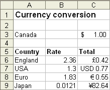
A4: B: =C$3/B6
This is another question about absolute and relative references because it's such an important point of using a spreadsheet. You must master this if you ever wish to use Excel efficiently. This formula can find the value of any Canadian currency into any other mentioned in the picture. The important point is that the formula can quickly be copied to the C6 to C9 cells and still work properly without changing it in any way.
A5: D: The split box
It was too easy. There are times when you need to compare values that are far away from each other. That's why it's an advantage to be able to split the screen in two vertically and/or horizontally and place the values close to each other on the screen. The split boxes help you do that easily.
A6: C:CTRL and Home
This combination of keys will always bring you back to the top of the sheet. The only time it will not work is if you "froze" part of the screen with the Freeze option under the Window menu. Excel will then place the cursor it the top cell of that frozen part of the sheet.
A7: B:CTRL
This key does allow you to select multiple ranges of cells so that youu can apply some options to them or use them for a chart. The Shift key allows you to select a single large range of cells. You only need to place the cursor on the first cell, press the Shift key and select the last cell of the range you need.
A8: B: F2
Other options you can use to change the content of a cell is to double click on the cell or selecting the cell and changing the content from the formula bar.
A9: C: AutoSum
First, there is no AutoCorrect option ... yet. The AutoSum option is probably the most often used option to create formulas. You can find other functions under the Insert and Function options.
A10: A: =A2*0.07 and B: =A2*7%
This is one of the rare times when there are two good ways to get the result you wish. You can either apply the decimal point or the percent character in this formula. The other two answers will give you the with the tax included. Don't expect two good answers in an exam.
A11: A: =If()
This is probably the most powerful function in Excel or any spreadsheet. It will show different results depending if the conditions were answered. It can be even more powerful when you include other functions such as AND() and OR() inside it . For example =if(and(condition1;condition2);If True;If false) or with other =if() inside the first if() =if(condition1;if(condition2;if true;if false);if false) . You can include up to six levels of if inside the first if function. But you may want to look at the =vlookup function before reaching that extreme.
Note:
TRUEFALSE is the equivalent of IF in Access that you can use in queries, forms and macros.
A12: A: =AND()
This function is used when you want to make sure that many conditions are fulfilled before showing a #TRUE# result.
A13: B: =OR(A1=2;A2=1)
All the conditions in the =and() function must be true before you get a #true# as a result. But that's not possible since the content of the A2 cell isn't equal to 2. The content of the A1 cell isn't superior to 1 either. So the result of this function will be false. But it could have been true if the condition was equal or superior to 1 (>=).
As for the =Or function, the A1=2 condition was false. But the A2=1 condition was true. So the result of this function is true.
A14: C: The values of the first column must be in descending order
The values must always be in ascending order. That's how the =vllokup() and =hlookup() can determine the lowest possible value to attain this level of the comparison table. It also determines the highest possible value for the level just below. The ascending order of the values help determine the top and bottom range for a level. That's not possible if the values are nor in that order.
A15: C: C
By using the =vlookup() function with the comparison table located between A4 and B8, all of the numbers between 70 and 79,9999 will give you a grade of "C". The first column will always show the lowest possible value to attain this "level". The letter "C" will appear as soon as the grade is superior to 70. The letter will change to "B" as soon as the grade is at 80 or above.
A16: E: None of the above
The fourth argument forces the function to find an exact value in the comparison table. Since Landry Transport isn't in the list, the function will return a #N/A (not applicable) result to show that this value is impossible under these conditions.
The result would be 5% if the fourth argument is TRUE. The function would try to place the value "Landry transport" between such and such values. It couldn't go any further than "Extermination Turcotte" since the value you're searching for isn't superior or equal to "Librairie Beauchemin". I must remind you that you can use this function in two ways: exact value or between such and such value. The values in the first column must be in ascending order.
A17: B: Solver
Scenarios are very practical when you want to compare many possibilities. Goal seek allows you to adjust the content of a cell so that you can attain your goal. But the Solver is there to help you optimize your model to achieve it's greatest possible value.
A18: B: False
The values that you enter in the scenarios have no impact on the worksheets. But the View scenarios option does impact your model. It replaces the content of the cells with the values of the scenarios. You may lose your original data if you don't cancel the view from the Edit menu. Another way is to create a scenario with the original values so that you may place them back in place. You also have to be sure that values of the scenarios do not replace the content of cells that contain formulas. Or else, the scenarios will erase the formulas and your model will become invalid. Be careful with this powerful option.
A19: D: None of the above
All of the answers above allow you to copy a cell or a range of cells. There's also the Copy option under the Edit menu. But it was too obvious to put it in the list. The Copy option is used often to copy text and formula. But you have to be very careful about relative and absolute references.
| You like what you read?
Share it with your friends. |